1 笨笨的孩子慢慢学stay hungry stay foolish 2 学习,思考,实践,改变

0%

排序算法复习

排序算法

排序算法在搜索中常用,因此非常重要。排序算法里包含了重要的分治的思想,就是在划分子问题上。归并排序将数据折半划分,快速排序将数据分成大数和小数部分,基数排序则每次都会按照关键码中的一个数字划分数据。

什么是稳定的排序:如果一种排序算法不会改变关键码值相同的记录的相对顺序,则称为稳定的。

三种基本的排序算法

插入排序

例子:每处理一次数据就把它和前面已经排序的子序列进行比较,再将它插入到前面的正确位置。算法里的Comp类要自己写,实现关键码比较大小,如int就直接比较大小,其他类别比较大小等等。

1
2
3
4
5
6
7
// C++
template <typename E, typename Comp>
void inssort(E A[], int n){
for (int i=1;i<n;i++)
for (int j=i; (j>0)&&(Comp::prior(A[j],A[j-1])); j--)
swap(A, j, j-1);
}
1
2
3
4
5
6
# python
def insert_sort(array):
for i in range(0,len(array)):
for j in range(i,0,-1):
if j>0 and array[j] < array[j-1]:
array[j],array[j-1] = array[j-1],array[j] # change the elem

这里最差的情况是每条记录都必须移动到最前面(如 array = [3,2,1,0]),空间复杂度由于并没有用其他临时数组,所以还是 $O(1)$,此时时间复杂度:

最佳情况就是每条记录都已经是有序的了,进入内部for循环就退出,于是此时的时间代价是 $\Theta(n)$

平均情况根据逆置来判断,逆置的数值(即数组中位于一个给定值之前的比它大的值的数目)决定比较与交换的次数。平均情况下,在数组的前i-1条记录中有一半关键码值比第i条记录的关键码值大。平均情况下,时间代价是最差情况的一半 $\Theta(n^2/4)$, 是稳定排序。

冒泡排序

例子:气泡冒上来的过程。从最后开始,比较相邻的,如果前面的比它大则交换。就像气泡逐渐被推到数组的顶部。

1
2
3
4
5
6
7
8
//C++
template <typename E,typename Comp>
void bubsort(E A[], int n){
for(int i=0; i<n-1;i++)
for(int j=n-1; j>i; j--)
if(Comp::prior(A[j],A[j-1]))
swap(A,j,j-1);
}
1
2
3
4
5
6
7
8
9
10
# python
def bubble_sort(array):
for i in range(0,len(array)-1):
flag = 0 # trace the exchange times
for j in range(len(array)-1,i,-1):
if array[j] < array[j-1]:
array[j], array[j - 1] = array[j - 1], array[j]
flag = 1
if(flag==0):
return

内层的for循环比较次数总会是 i,因此最差时间代价是:$\sum_{i=1}^n i \approx n^2/2 = \Theta(n^2)$ ,平均也是类似插入排序$\Theta(n^2)$,它是稳定的排序。

修改冒泡排序以跟踪其执行的交换次数。 如果数组已经按排序顺序排列,并且冒泡排序不进行交换,则算法可以在经过一遍后终止。在最佳情况下复杂度是 $\Theta(n)$ 。

冒泡排序相对于大多数其他算法(甚至是快速排序,但不是插入排序)具有的唯一显着优势是,该算法内置了检测列表是否被有效排序的功能。

选择排序

选择排序就是选择数组中第i小的记录,并把该记录放到数组的第i个位置上,只需一次交换,不稳定排序。

数组中的相邻元素两两比较,按照小元素在前来交换,每一轮结束后最小的元素被交换到了最后一位。

1
2
3
4
5
6
7
8
9
10
template <typename E,typename Comp>
void selsort(E A[], int n){
for(int i=0; i<n-1; i++){
int lowindex = i;
for(int j=n-1; j>i ; j--)
if(Comp::prior(A[j], A[lowindex]))
lowindex = j;
swap(A,i,lowindex);
}
}
1
2
3
4
5
6
7
8
9
# python

def select_sort(array):
for i in range(0,len(array)-1):
lowindex = i
for j in range(len(array)-1, i, -1):
if array[j] < array[lowindex]:
lowindex = j
array[i], array[lowindex] = array[lowindex], array[i]
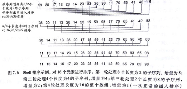
比较的次数是 $\Theta(n^2)$ ,但交换的次数比冒泡排序少很多,对于那些做交换花费时间多的问题是更好的。

改进的排序

shellsort

它在不相邻的记录之间进行比较与交换。shell排序利用了插入排序的最佳时间代价特性。他将序列分成多个子序列,然后分别对子序列进行排序,最后将子序列组合起来。由于实现了元素的跳跃式移动(希尔排序会用较大的步长移动数据),使排序效率提高。如下图:图中的增量序列就是8,4,2,1。最后一轮将是一次“正常的”插入排序,因为此时序列整体基本上有序,故用插入排序的复杂度相对较小。

shellsort增量选择3的时候,效果较好,平均运行时间复杂度是$\Theta(n^{1.5})$ 。

相同的元素可能在各自的插入排序中移动, 是不稳定排序。在中等大小规模的数据上表现良好。

20200310shellsort

1
2
3
4
5
6
7
8
9
10
11
12
13
14
15
16
17
18
19
20
21
22
23
24
25
26
27
28
29
30
//shellsort
template <typename E>
void insort(E A[],int n, int increment){
for (int i=increment; i<n; i+=increment) {
for (int j=i; (j>=increment)&&(A[j]<A[j-increment]); j-=increment) {
E temp = A[j];
A[j] = A[j-increment];
A[j-increment] = temp;
}
}
}

template <typename E>
void shellsort(E A[],int n){
for (int i=n/2; i>2; i/=2) {
for (int j=0; j<i; j++) {
insort<E>(&A[j], n-j, i);//A[j] is the start address 偏移,巧妙
}
}
insort<E>(A, n, 1);
}

int main(){
int num[16] = {59,20,17,13,28,14,23,83,36,98,11,70,65,41,42,15};
shellsort<int>(num, 16);
for (auto n:num) {
cout<<n<<endl;
}
return 0;
}

Python:

1
2
3
4
5
6
7
8
9
10
11
12
def shell_sort(array):
n = len(array)
gap = n // 2
while gap > 0:
for i in range(gap,n):
temp = array[i]
j = i
while j >= gap and array[j-gap] > temp:
array[j] = array[j-gap]
j-=gap
array[j] = temp
gap //= 2
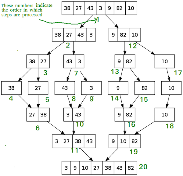
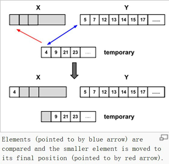
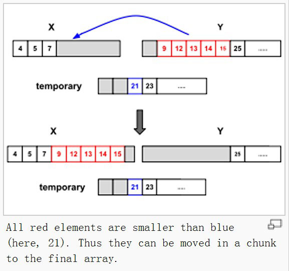
mergesort

来源于分治的思想,在排序问题上分治的思想体现在把待排序的列表分成片段,先处理片段,然后将片段重组。

伪代码的提现其思想:

1
2
3
4
5
6
List mergesort(List inlist){
if(inlist.length() <= 1) return inlist;
List L1 = half of the list;
List L2 = other half of the list;
return mergesort(mergesort(L1),mergesort(L2));
}

20200310Merge-Sort

当输入的待排序数据存储在链表中时,归并排序是一个很好的选择。

两个指针,最初分别为两个已经排序序列的起始位置。比较两个指针所指向的元素,选择相对小的元素放入到合并空间,并移动指针到下一位置。重复直到某一指针达到序列尾,剩下的元素直接放入到合并的片段里。

1
2
3
4
5
6
7
8
9
10
11
12
13
14
15
16
17
18
19
20
21
22
23
24
25
26
27
28
29
30
31
32
33
#include <iostream>
using namespace std;

template <typename E>
void mergesort(E A[],E temp[], int left, int right){
if (left == right) {
return;
}
int mid = left + (right-left)/2;
mergesort<E>(A, temp, left, mid);
mergesort<E>(A, temp, mid+1, right);
//then merge, temp[] is the auxiliary array
for (int i=left; i<=right; i++) {
temp[i] = A[i];
}
int i1 = left;
int i2 = mid+1;
for (int curr=left; curr<=right; curr++) {
if (i1 == mid+1) A[curr] = temp[i2++]; //left all < right
else if(i2 > right) A[curr] = temp[i1++]; //right all < left
else if (temp[i1] < temp[i2]) A[curr] = temp[i1++];// smaller one is put into A
else A[curr] = temp[i2++];
}
}
int main(){
int num[16] = {59,20,17,13,28,14,23,83,36,98,11,70,65,41,42,15};
int temp[16] = {0};
mergesort<int>(num, temp, 0, 15);
for (auto n:num) {
cout<<n<<endl;
}
return 0;
}

当被排序元素的数目是n时,递归的深度是$logn$ ,第一层递归是对长度为n的数组排序,下一层是对2个长度为n/2的子数组排序……,在所有$logn$ 层递归中,每一层都需要$\Theta(n)$ 时间代价,因此总时间代价都是$n log(n)$。由于需要temp数组做临时存储,空间复杂度是$\Theta(n)$.

python版本代码可以参考 https://www.geeksforgeeks.org/python-program-for-merge-sort/

quicksort

快速排序不需要额外的空间,典型应用是Unix系统调用库里的qsort函数。快速排序选定一个轴值,数组在小于轴值的放在左边,大于的放在右边。这被称为数组的一个划分 partition。快速排序最差情况是当轴值每次都不能把数组划分得很好,下一次处理子问题规模只比原来的问题规模减少1,时间代价是$\Theta(n^2)$ ,最佳和平均复杂度是$\Theta(n logn)$ 。2,由于递归调用,空间复杂度是$\Theta(logn)$

快排为什么这么快?

1
2
3
4
5
6
7
8
9
10
11
12
13
14
15
16
17
18
19
20
21
22
23
24
25
26
27
28
29
30
#include <iostream>
#include <vector>
#include <queue>
using namespace std;

void swap(int A[], int i, int j)
{
int temp = A[i];
A[i] = A[j];
A[j] = temp;
}

int partition(int A[],int l, int r, int& pivot){
do{
while(A[++l] > pivot); //move the index
while((l<r) && (A[--r] < pivot));
swap(A,l,r);
}while(l<r);
return l;
}

void myqsort(int A[],int i,int j){
if (i >= j) return;
int pivotIndex = (i+j)/2; //这里可以写一个findpivot函数,三者取中(三个随机值的中间)
swap(A,pivotIndex,j);
int k = partition(A,i-1,j,A[j]); //k is the start of the left half
swap(A,k,j);// 轴值就在k位置,就是最终排序好的数组中的位置
myqsort(A,i,k-1);
myqsort(A,k+1,j);
}

这里面的改进可以从pivotIndex的设置,以及递归到一个较小的数组的时候采用插入排序(基本有序的小数组很适合)等。

Python版本:更清晰一点,把轴值设置为左边第一个。

1
2
3
4
5
6
7
8
9
10
11
12
13
14
15
16
17
def quick_sort(array, left, right):
if left >= right:
return
low = left
high = right
key = array[low]
while left < right:
while left < right and array[right] > key:
right -= 1
array[left] = array[right]
while left < right and array[left] <= key:
left += 1
array[right] = array[left]
array[right] = key

quick_sort(array, low, left - 1)
quick_sort(array, left + 1, high)

heapsort

堆是一棵完全二叉树,可以用数组来实现。参考 数组实现堆)

堆可以用来排序,适合于那些数据集太大而不适合在内存中排序的例子。

1
2
3
4
5
6
7
template <typename E>
void heapsort(E A[], int n){
E maxval;
heap<E> Heap(A,n,n); //build the heap
for (int i=0; i<n ; i++)
maxval = Heap.removefirst();
}

建堆需要$\Theta(n)$,且n次取堆的最大元素要用$\Theta(logn)$ 时间,因此时间代价是$nlogn$。但堆排序一般情况下比快排在常熟因子上慢。

为什么堆排比快排慢?堆排序将最大值取走后要调整结构,用堆底元素替换堆顶元素,然后那最后一个元素从顶上往下滑到恰当的位置(重新使堆最大化)。其实这里堆底的元素肯定很小,将它拿到堆顶和原本属于最大元素的两个子节点比较,比他们都大的可能性是很小的。这一次比较的结果就是概率不均等的,这次比较就很有可能是无效的,堆顶元素很有可能继续下移比较。

Python实现:

1
2
3
4
5
6
7
8
9
10
11
12
13
14
15
16
17
18
19
20
21
22
23
24
25
26
27
28
29
30
# To heapify subtree rooted at index i , n is size of heap
def heapify(array,n,i):
largest = i # init largest as root
l = 2 * i + 1
r = 2 * i + 2

# See if left child of root exists and is greater than root
if l < n and array[i] < array[l]:
largest = l
# See if right child of root exists and is greater than root
if r < n and array[largest] < array[r]:
largest = r

# Change root, if needed
if largest != i:
array[i], array[largest] = array[largest], array[i] # swap
# Heapify the root
heapify(array, n, largest)


# The main function to sort an array of given size
def heapSort(arr):
n = len(arr)
# Build a maxheap.
for i in range(n, -1, -1):
heapify(arr, n, i)
# One by one extract elements
for i in range(n - 1, 0, -1):
arr[i], arr[0] = arr[0], arr[i] # swap
heapify(arr, i, 0)
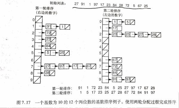
计数排序 / 分配排序Binsort

1
2
for (int i=0;i<n;i++)
B[A[i]] = A[i];

这里的关键码用来确定一个记录在排序中的最后的位置,关键码将记录放到盒子里,是分配排序的一个基本例子。比如数组[0,3,4,2,1] 经过一遍之后,B array 就直接把值放到了该放的地方了。

但这里它只能用于对一个从0到n-1的序列进行排序,而且还有重复的问题待处理。如果数组B变成一个链表数组,将所有的关键码i的值放到B[i] 盒子里,这就解决了重复的问题。另一个扩展是允许关键码大于n。

1
2
3
4
5
6
7
8
9
10
11
12
13
14
15
16
17
18
19
20
21
22
23
24
#include <iostream>
#include <list>
using namespace std;

const int MaxKeyValue = 100; // 0<=A[i]<=50
void Binsort(int A[],int n){ // n is the A.length
if(n<=0) return;
list<int> B[MaxKeyValue];
for (int i=0; i<n; i++) {
B[A[i]].push_back(A[i]);
}
for (int i=0; i<MaxKeyValue; i++) {
if (B[i].size() != 0) {
for (list<int>::iterator it=B[i].begin(); it!=B[i].end(); ++it) {
cout<<*it<<',';
}
}
}
}
int main(){
int num[16] = {59,20,17,13,28,14,23,83,36,98,11,70,65,41,42,15};
Binsort(num,16);
return 0;
}

这里也可以优化一些,计数排序:B[A[i]] 存储 A[i] 值出现的次数。这样最好遍历一遍B,再根据次数,输出下标值,即排序后的A[i]。但以上设计的缺陷是MaxKeyValue太大了,如果是$n^2$ , 那么时间代价就是 $\Theta(n^2)$ ,而且所用空间也更大了。

桶排序/基数排序

进一步改进前面的Binsort为桶式排序Bucketsort,每一个盒子并非与一个关键码值联系,而是与一组关键码有关。记录放到“桶”中后,再借用其他排序对桶里的记录排序。

eg:有10个盒子,首先可以把记录的关键码对10取模的结果赋值到盒子里,这样每个关键码都以其个位为标准放到10个不同的盒子里。然后按顺序再收集这些记录,按照最高位(十位)对他们进行排序。如图:

20200310BucketSort

对于n长的序列,假设基数是r,这个算法需要k轮,每一轮分配的时间是$\Theta(n+r)$ ,总时间代价是$\Theta(nk + rk)$, k是与关键码的长度有关。因此平均时间复杂度是$\theta(n)$,空间复杂度是用于计数的cnt数组和Bin辅助数组带来的 $\Theta(n + k)$

1
2
3
4
5
6
7
8
9
10
11
12
13
14
15
16
17
18
19
20
21
22
23
24
25
26
27
28
29
30
31
32
33
34
35
36
37
38
39
40
41
42
43
//每一轮分配结束时,记录都被复制回原数组
void radix(int* A, int* Bin,int n,int k,int r,int cnt[]){
//n is the size of A
//k is the digit of A[max], r is Cardinality 10 (make r from 1 to 10 to 100)
//cnt[i] stores occurrences of records in bin[i]
int j;
for (int i=0,rtoi=1; i<k; i++,rtoi*=r) {
for (j=0; j<r; j++) cnt[j] = 0; //init cnt,roti save the r^i

//count the number of records for each bin on this pass
for (j=0; j<n; j++) cnt[(A[j] / rtoi) % r]++;

//index of B: cnt[j] will be index for last slot of bin j
for (j=1; j<r; j++) cnt[j] = cnt[j-1] + cnt[j];

//put records into bins, work from bottom of each bin
//since bins fill from bottom, j counts downwards
for (j=n-1; j>=0; j--) {
Bin[--cnt[ (A[j] / rtoi) % r] ] = A[j];
}

//copy B back to A
for (j=0; j<n; j++) {
A[j] = Bin[j];
}
cout<<endl;
}
}

int main(){
//n is the size of A,k is the digit of A[max], r is Cardinality 10 (make r from 1 to 10 to 100)
int n = 12;
int k = 2;
int r = 10;
int A[12] = {27,91,1,97,17,23,84,28,72,5,67,25};
int B[12] = {0,0,0,0,0,0,0,0,0,0,0,0};
int cnt[10] = {0};
radix(A,B,n,k,r,cnt);
for (int i=0; i<n; i++) {
cout<<A[i]<<" ";
}
return 0;
}

在此记录一个degub情况:上面有个情况是cnt的计数数组,判断A数组里的数应该放到哪个合适的位置出了个bug,cnt被A[j] = 72的时候篡改了。这里编程规范得注意,好好初始化,因为没指定数组长度,程序执行过程中很有可能地址错乱!!!

其他内嵌算法

timsort

这是Python的内嵌排序算法,是 list.sort 的默认实现。

它结合了合并排序(merge sort)和插入排序(insertion sort)而得出的排序算法。

思想:TimSort 算法为了减少对升序部分的回溯和对降序部分的性能倒退,将输入按其升序和降序特点进行了分区。该算法找到数据中已经排好序的块 - 分区,每一个分区叫一个run,然后按规则合并这些run,合并的结果保存到栈中。

关于run:现实中的大多数据通常是有部分已经排好序的,以一个分区run作为排序单位更好。

20200423sort_run

每次拿一个 run 出来进行归并。每次归并会将两个 run 合并成一个 run。

run的最小长度

run是已经排好序的一块分区,run长度不同,Timesort根据run的长度来选择排序的策略。

例如如果run的长度小于某一个值,则会选择插入排序算法来排序。

合并run

合并run的原则是 run合并的技术要保证有最高的效率。当Timsort算法找到一个run时,会将该run在数组中的起始位置和run的长度放入栈中,然后根据先前放入栈中的run决定是否该合并run。Timsort不会合并在栈中不连续的run。

Timsort会合并在栈中2个连续的run。X、Y、Z代表栈最上方的3个run的长度(图2),当同时不满足下面2个条件是,X、Y这两个run会被合并,直到同时满足下面2个条件,则合并结束:

(1) X>Y+Z

(2) Y>Z

如果X<Y+Z,那么X+Y合并为一个新的run,然后入栈。重复上述步骤,直到同时满足上述2个条件。当合并结束后,Timsort会继续找下一run,然后找到以后入栈,重复上述步骤,及每次run入栈都会检查是否需要合并2个run。

简单的合并算法是用简单插入算法,依次从左到右或从右到左比较,然后合并2个run。

20200423sort_run_merge

Timsort用\二分插入算法(binary merge sort)。**先用二分查找算法/折半查找算法(binary search)找到插入的位置,然后在插入。

20200423sort_run_merge2

由于Timsort算法利用了现实中大多数数据中会有一些排好序的区,所以Timsort会比$O(nlogn)$快些。

总结

排序算法 平均时间复杂度 最坏时间复杂度 最好时间复杂度 空间复杂度 稳定性
冒泡排序 O(n²) O(n²) O(n) O(1) 稳定
直接选择排序 O(n²) O(n²) O(n²) O(1) 不稳定
直接插入排序 O(n²) O(n²) O(n) O(1) 稳定
快速排序 O(nlogn) O(n²) O(nlogn) O(nlogn) 不稳定
堆排序 O(nlogn) O(nlogn) O(nlogn) O(1) 不稳定
希尔排序 O(n^1.5) O(n log² n) O(n log²n) O(1) 不稳定
归并排序 O(nlogn) O(nlogn) O(nlogn) O(n) 稳定
计数排序 O(n+k) O(n+k) O(n+k) O(n+k) 稳定
基数排序 O(N*M) O(N*M) O(N*M) O(M) 稳定

Reference

1,《数据结构与算法分析》 Clifford A. Shaffer 等

2,百度百科)

3, 机器之心 Timsort

4,GeeksforGeeks-Python实现mergesort

5,TimSort原理介绍